Inferring probabilities, a second example of Bayesian calculations
Oct 24, 2014
warning
This post is more than 5 years old. While math doesn't age, code and operating systems do. Please use the code/ideas with caution and expect some issues due to the age of the content. I am keeping these posts up for archival purposes because I still find them useful for reference, even when they are out of date!
In this post I will focus on an example of inferring probabilities given a short data series. I will start by tackling the theory of how to do the desired inference in a Bayesian way and will end by implementing the theory in Python so that we can play around with the ideas. In an attempt to keep the post more accessible, I will only consider a small set of candidate probabilities. This restriction allows me to minimize the mathematical difficulty of the inference and still obtain really cool results, including nice plots of the prior, likelihood and posterior.
If the content below seems unfamiliar try reading previous posts that provide some of the needed background to understand the current post:
- Joint, conditional and marginal probabilities
- Medical tests, a first example of Bayesian calculations
Check those out to get some background, or jump right in. To be concrete, I'll consider the following scenario:
-
A computer program outputs a random string of \( 1 \)s and \( 0 \)s --
we'll use
numpy.random.choicein Python as our source for data. For example, one sample output could be: \[ D = 0000110001 \] - The goal will be to infer the probability of a \( 0 \) that the program is using to produce \( D \). We'll use the notation \( p_{0} \) for the probability of a \( 0 \). Of course this also means that the probability of a \( 1 \) must be \( p_{1} = 1 - p_{0} \).
- As discussed above, we will only consider a set of candidate probabilities. To be concrete, let's use the candidates \( p_{0} = 0.2, 0.4, 0.6, 0.8 \) for the data series above. How do we sensibly choose among these possibilities and how certain are we of the result?
Likelihood
My starting point is to write down the probability of the data series as if I knew the probability of a \( 0 \) or a \( 1 \). Of course I don't know these probabilities-- finding these probabilities is our goal-- but trust me, this is leading somewhere useful. For example, the probability of our example data series, without being specific about the value of \( p_{0} \), can be written:
\[ \begin{array}{ll} P(D=0000110001 \vert p_{0} ) & = & p_{0} \times p_{0} \times p_{0} \\ & \times & p_{0} \times (1-p_{0}) \times (1-p_{0}) \\ & \times & p_{0} \times p_{0} \times p_{0} \\ & \times & (1-p_{0}) \end{array} \]where I've used \( p_{1} = 1 - p_{0} \) to write the probability in terms of just \( p_{0} \). I can also collect terms and write the above probability in a more compact way:
\[ P(D=0000110001 \vert p_{0} ) = p_{0}^{7} \times (1-p_{0})^{3} \]Technical aside: the form of the probabilities given above is called a Bernoulli Process (as opposed to a Bernoulli Trial or Binomial Distribution ). I can also write this probability in a very general way, without being specific about the data series \( D \) or probability \( p_{0} \), as:
\[ P(D \vert p_{0}) = p_{0}^{n_{0}} \times (1 - p_{0})^{n_{1}} \]\( n_{0} \) and \( n_{1} \) denote the number of \( 0 \)s and \( 1 \) s in the data series I am considering.
I can connect the general form to a specific example by substituting the relevant counts and probabilities. I'll start by calculating the likelihood values for the data series and probabilities given above:
\[ \begin{array}{ll} P(D=0000110001 \vert p_{0}=0.2) & = & 0.2^{7} \times (1-0.2)^{3} \\[1em] & = & 6.55360 \times 10^{-6} \\[1.5em] P(D=0000110001 \vert p_{0}=0.4) & = & 0.4^{7} \times (1-0.4)^{3} \\[1em] & = & 3.53894 \times 10^{-4} \\[1.5em] P(D=0000110001 \vert p_{0}=0.6) & = & 0.6^{7} \times (1-0.6)^{3} \\[1em] & = & 1.79159 \times 10^{-3} \\[1.5em] P(D=0000110001 \vert p_{0}=0.8) & = & 0.8^{7} \times (1-0.8)^{3} \\[1em] & = & 1.67772 \times 10^{-3} \end{array} \]Inspecting the results, I see that \( p_{0}=0.6 \) produces the highest likelihood, slightly beating out \( p_{0}=0.8 \). A couple of things to note here are:
- I have the maximum likelihood value (among the values considered). I could provide the answer \( p_{0}=0.6 \) and be done.
- The sum of the probabilities (likelihoods) is not 1. This means that I do not have a properly normalized probability mass function (pmf) with respect to \( p_{0} \), the parameter that I am trying to infer. A goal of Bayesian inference is to provide a properly normalized pmf for \( p_{0} \), called the posterior.
The ability to do the above calculations puts me in good shape to apply Bayes' Theorem and obtain the desired posterior pmf. Before moving on to Bayes' Theorem I want to re-emphasize the general form of the likelihood:
\[ P(D \vert p_{0}) = p_{0}^{n_{0}} \times (1 - p_{0})^{n_{1}} \]It will also be useful to have the log-likelihood written down:
\[ \begin{array}{ll} \ln P(D \vert p_{0}) & = & n_{0} \times \ln(p_{0}) \\ & + & n_{1} \times \ln(1 - p_{0}) \end{array} \]because this form adds to the numerical stability when I create some Python code below. If you are rusty with logarithms, check out wikipedia logarithm identities for examples of how to get from the likelihood to the log-likelihood. To be clear, I am using natural (base-e) logarithms, that is \( \log_{e}(x) = \ln(x) \).
Prior
I've already decided on part of the prior-- I've done this by choosing \( p_{0} \in \{ 0.2, 0.4, 0.6, 0.8 \} \) as the set of probabilities that I will consider. All that is left is to assign prior probabilities to each candidate \( p_{0} \) so that I can start with a properly normalized prior pmf. Let's say that I have no reason to prefer any of the candidates and make them equally probable, a priori:
\[ \begin{array}{ll} P(p_{0}=0.2 \vert A1) & = & 0.25 \\ P(p_{0}=0.4 \vert A1) & = & 0.25 \\ P(p_{0}=0.6 \vert A1) & = & 0.25 \\ P(p_{0}=0.8 \vert A1) & = & 0.25 \\ \end{array} \]where use \( A1 \) to denote the assumptions that I've made. The above information makes up my prior pmf.
Bayes' Theorem and the Posterior
Next I employ the likelihood and prior pmf defined above to make an inference about the underlying value of \( p_{0} \). That is, I will use Bayes' Theorem to calculate the posterior pmf given the likelihood and prior. The posterior has the form
\[ P(p_{0} \vert D, A1) \]In words, this is the probability (pmf) of \( p_{0} \) given data series \( D \) and assumptions \( A1 \). Hey, that's just what I want! I can calculate the posterior using Bayes' Theorem:
\[ \color{blue}{P(p_{0} \vert D, A_{1})} = \color{black}{\frac{ P(D \vert p_{0}) \color{red}{P(p_{0}\vert A_{1})} }{ \sum_{ \hat{p_{0}} } P(D \vert p_{0} = \hat{p_{0}}) \color{red}{P(p_{0} = \hat{p_{0}} \vert A_{1})} } } \]where the prior \( \color{red}{P(p_{0} \vert A_{1})} \) is red, the likelihood \( P(D\vert p_{0}) \) is black, and the posterior \( \color{blue}{P(p_{0} \vert D, A_{1})} \) is blue. This allows my information about \( p_{0} \) to updated from assumptions ( \( A_{1} \) ) to assumptions + data ( \( D, A_{1}\) ):
\[ \color{red}{P(p_{0} \vert A_{1})} \color{black}{\rightarrow} \color{blue}{P(p_{0} \vert D, A_{1})} \]I can simplify the look of Bayes' Theorem by defining the marginal likelihood, or evidence:
\[ P(D \vert A_{1}) = \sum_{ \hat{p_{0}} } P(D \vert p_{0} = \hat{p_{0}}) \color{red}{P(p_{0} = \hat{p_{0}} \vert A_{1})} \]This lets me write Bayes' Theorem in the following form:
\[ \color{blue}{P(p_{0} \vert D, A_{1})} \color{black}{ = \frac{ P(D \vert p_{0}) \color{red}{P(p_{0} \vert A_{1})} }{ P(D \vert A_{1}) } } \]The posterior should really be thought of as a set of equations, one for each candidate value of \( p_{0} \), just like we had for the likelihood and the prior.
Finally, for the theory, I finish off our example and calculate the posterior pmf for \( p_{0} \). Let's start by calculating the evidence (I know all the values for the likelihood and prior from above):
So, the denominator in Bayes' Theorem is equal to \( 9.57440e-04 \). Now, complete the posterior pmf calculation.
- First, \( P(p_{0} = 0.2 \vert D=0000110001, A_{1}) \)
\[ \begin{array}{ll} & = & \cfrac{ P(D=0000110001 \vert p_{0} = 0.2) P(p_{0} = 0.2 \vert A_{1}) }{ P(D=0000110001 \vert A_{1}) } \\[1em] & = & \cfrac{6.55360e-06 \times 0.25}{9.57440e-04} \\[1em] & = & 1.78253e-03 \end{array} \] - Second, \( P(p_{0} = 0.4 \vert D=0000110001, A_{1}) \)
\[ \begin{array}{ll} & = & \cfrac{ P(D=0000110001 \vert p_{0} = 0.4) P(p_{0} = 0.4 \vert A_{1}) }{ P(D=0000110001 \vert A_{1}) } \\[1em] & = & \cfrac{3.53894e-04 \times 0.25}{9.57440e-04} \\[1em] & = & 9.62567e-02 \end{array} \] - Third, \( P(p_{0} = 0.6 \vert D=0000110001, A_{1}) \)
\[ \begin{array}{ll} & = & \cfrac{ P(D=0000110001 \vert p_{0} = 0.6) P(p_{0} = 0.6 \vert A_{1}) }{ P(D=0000110001 \vert A_{1}) } \\[1em] & = & \cfrac{1.79159e-03 \times 0.25}{9.57440e-04} \\[1em] & = & 4.87299e-01 \end{array} \] - Finally, \( P(p_{0} = 0.8 \vert D=0000110001, A_{1}) \)
\[ \begin{array}{ll} & = & \cfrac{ P(D=0000110001 \vert p_{0} = 0.8) P(p_{0} = 0.8 \vert A_{1}) }{ P(D=0000110001 \vert A_{1}) } \\[1em] & = & \cfrac{1.67772e-03 \times 0.25}{9.57440e-04} \\[1em] & = & 4.56328e-01 \end{array} \]
Summing Up
Before moving on to the Python code, let's go over the results a bit. Using the data series and Bayes' Theorem I've gone from the prior pmf
to the posterior pmf (I'll shorten the data series in the notation below)
In a Bayesian setting, this posterior pmf is the answer to our inference of \( p_{0} \), reflecting our knowledge of the parameter given the assumptions and data. Often people want to report a single number but this posterior reflects a fair amount of uncertainty. Some options are:
- Report the maximum a posteriori value of \( p_{0} \)-- in this case \( 0.6 \).
- Report the posterior mean, or the posterior median-- using the posterior pmf to calculate.
- Include a posterior variance or credible interval to describe uncertainty in the estimate.
However the inference is reported, communicating the uncertainty is part of the job. In practice, plots of the posterior really help with the task. So, let's leave theory and implement these ideas in Python.
Writing the inference code in Python
This code will be available as a single Python script,
ex001_bayes.py, at this
github gist
(edit: changed to gist Mar 5, 2015). You should grab it and try to
following along.
First, the code has some imports -- just numpy and matplotlib. I will also use a nice ggplot style to make the plots look really nice.
from __future__ import division, print_function
import numpy as np
import matplotlib.pyplot as plt

# use matplotlib style sheet
try:
    plt.style.use('ggplot')
except:
    # version of matplotlib might not be recent
    pass
First, I make a class to deal with the likelihood. The
class takes the
data series and provides an interface for computing the likelihood for a given
probability \( p_{0} \). You should be able to find the
log-likelihood equation in the
_process_probabilities() method (with
some care taken for edge cases).
class likelihood:
    def __init__(self, data):
        """Likelihood for binary data."""
        self.counts = {s:0 for s in ['0', '1']}
        self._process_data(data)

    def _process_data(self, data):
        """Process data."""
        temp = [str(x) for x in data]
        for s in ['0', '1']:
            self.counts[s] = temp.count(s)

        if len(temp) != sum(self.counts.values()):
            raise Exception("Passed data is not all 0`s and 1`s!")

    def _process_probabilities(self, p0):
        """Process probabilities."""
        n0 = self.counts['0']
        n1 = self.counts['1']

        if p0 != 0 and p0 != 1:
            # typical case
            logpr_data = n0*np.log(p0) + \
                         n1*np.log(1.-p0)
            pr_data = np.exp(logpr_data)
        elif p0 == 0 and n0 != 0:
            # p0 can't be 0 if n0 is not 0
            logpr_data = -np.inf
            pr_data = np.exp(logpr_data)
        elif p0 == 0 and n0 == 0:
            # data consistent with p0=0
            logpr_data = n1*np.log(1.-p0)
            pr_data = np.exp(logpr_data)
        elif p0 == 1 and n1 != 0:
            # p0 can't be 1 if n1 is not 0
            logpr_data = -np.inf
            pr_data = np.exp(logpr_data)
        elif p0 == 1 and n1 == 0:
            # data consistent with p0=1
            logpr_data = n0*np.log(p0)
            pr_data = np.exp(logpr_data)

        return pr_data, logpr_data

    def prob(self, p0):
        """Get probability of data."""
        pr_data, _ = self._process_probabilities(p0)

        return pr_data

    def log_prob(self, p0):
        """Get log of probability of data."""
        _, logpr_data = self._process_probabilities(p0)

        return logpr_data
Next I create a class for the prior pmf. Given a list of candidate values for \( p_{0} \), this creates a uniform prior by default. If something else is desired, a dictionary of prior probabilities can be passed to override this default. I'll do an example below.
class prior:
    def __init__(self, p_list, p_probs=None):
        """The prior.

        p_list: list of allowed p0's
        p_probs: [optional] dict of prior probabilities
                 default is uniform
        """
        if p_probs:
            # make sure prior is normalized
            norm = sum(p_probs.values())
            self.log_pdict = {p:np.log(p_probs[p]) - \
                                np.log(norm) for p in p_list}
        else:
            n = len(p_list)
            self.log_pdict = {p:-np.log(n) for p in p_list}

    def __iter__(self):
        return iter(sorted(self.log_pdict))

    def log_prob(self, p):
        """Get log prior probability for passed p0."""
        if p in self.log_pdict:
            return self.log_pdict[p]
        else:
            return -np.inf

    def prob(self, p):
        """Get prior probability for passed p0."""
        if p in self.log_pdict:
            return np.exp(self.log_pdict[p])
        else:
            return 0.0
Finally I construct a class for the posterior that takes the
data series and an instance of the prior
class and constructs the posterior pmf. A
plot() method provides a really nice
visualization of the inference, including plots of the prior,
likelihood, and posterior.
Notice that all of the calculations for the posterior are done using log-probabilities. This is absolutely necessary for numerical accuracy because the probabilities can vary greatly and some are extremely small.
class posterior:
    def __init__(self, data, prior):
        """The posterior.

        data: a data sample as list
        prior: an instance of the prior class
        """
        self.likelihood = likelihood(data)
        self.prior = prior

        self._process_posterior()

    def _process_posterior(self):
        """Process the posterior using passed data and prior."""

        numerators = {}
        denominator = -np.inf
        for p in self.prior:
            numerators[p] = self.likelihood.log_prob(p) + \
                            self.prior.log_prob(p)

            if numerators[p] != -np.inf:
                # np.logaddexp(-np.inf, -np.inf) issues warning
                # skip-- this is adding 0 + 0
                denominator = np.logaddexp(denominator,
                                           numerators[p])

        # save denominator in Bayes' Theorem
        self.log_marg_likelihood = denominator

        # calculate posterior
        self.log_pdict = {}
        for p in self.prior:
            self.log_pdict[p] = numerators[p] - \
                                self.log_marg_likelihood

    def log_prob(self, p):
        """Get log posterior probability for passed p."""
        if p in self.log_pdict:
            return self.log_pdict[p]
        else:
            return -np.inf

    def prob(self, p):
        """Get posterior probability for passed p."""
        if p in self.log_pdict:
            return np.exp(self.log_pdict[p])
        else:
            return 0.0

    def plot(self):
        """Plot the inference resuults."""

        f, ax= plt.subplots(3, 1, figsize=(8, 6), sharex=True)

        # get candidate probabilities from prior
        x = [p for p in self.prior]

        # plot prior
        y1 = np.array([self.prior.prob(p) for p in x])
        ax[0].stem(x, y1, linefmt='r-', markerfmt='ro', basefmt='w-')
        ax[0].set_ylabel("Prior", fontsize=14)
        ax[0].set_xlim(-0.05, 1.05)
        ax[0].set_ylim(0., 1.05*np.max(y1))

        # plot likelihood
        y2 = np.array([self.likelihood.prob(p) for p in x])
        ax[1].stem(x, y2, linefmt='k-', markerfmt='ko', basefmt='w-')
        ax[1].set_ylabel("Likelihood", fontsize=14)
        ax[1].set_xlim(-0.05, 1.05)
        ax[1].set_ylim(0., 1.05*np.max(y2))

        # plot posterior
        y3 = np.array([self.prob(p) for p in x])
        ax[2].stem(x, y3, linefmt='b-', markerfmt='bo', basefmt='w-')
        ax[2].set_ylabel("Posterior", fontsize=14)
        ax[2].set_xlabel("Probability of Zero", fontsize=14)
        ax[2].set_xlim(-0.05, 1.05)
        ax[2].set_ylim(0., 1.05*np.max(y3))

        plt.tight_layout()
        plt.show()
Examples
Let's test out the code. First, I will replicate the example we did in the theory example to make sure all is well:
# data
data1 = [0,0,0,0,1,1,0,0,0,1]

# prior
A1 = prior([0.2, 0.4, 0.6, 0.8])

# posterior
post1 = posterior(data1, A1)
post1.plot()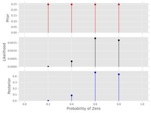
Notice how the posterior pmf nicely shows that both \( p_{0}=0.6 \) and \( p_{0}=0.8 \) have substantial probability-- there is uncertainty here! That makes sense because we only have a data series of length 10 and the are only four candidate probabilities. Also, notice:
- The sums of all stems in the prior and the posterior sum to 1, reflecting that these are proper pmfs.
- The likelihood does not have this property -- look at the scale on the y-axis. This gets even worse when we consider a longer data series below.
- Because the prior was uniform, the posterior shape looks just like the likelihood.
Next, let's consider setting a strong prior -- preferring one value of \( p_{0} \). Using our Python code it is easy to see the effect of this prior on the resulting posterior:
# prior -- will be normalized by class
A2 = prior([0.2, 0.4, 0.6, 0.8],
           {0.2:1, 0.4:20, 0.6:1, 0.8:1})

# posterior
post2 = posterior(data1, A2)
post2.plot()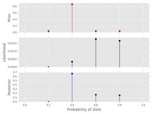
Notice the following things:
- The posterior and the likelihood no longer have the same shape. The strong prior affects the inference-- we should have a really good reason to use this prior!
- The posterior probabilities of \( p_{0}=0.2,0.4 \) have both decreased relative to their prior probabilities because of their low likelihood for the provided data series. In a similar manner, the posterior probabilities of \( p_{0}=0.6, 0.8 \) have increased relative to their prior probabilities. This makes sense because of the prior and the data provided!
Finally, let's do a quick example with more candidate probabilities, 100 in this case, and a longer data series.
# set probability of 0
p0 = 0.23
# set rng seed to 42
np.random.seed(42)
# generate data
data2 = np.random.choice([0,1], 500, p=[p0, 1.-p0])

# prior
A3 = prior(np.arange(0.0, 1.01, 0.01))

# posterior
post3 = posterior(data2, A3)
post3.plot()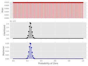
Notice a few things:
- The posterior has a nice smooth shape-- this looks like I treated the probability as a continuous value (I'll do that in a future post).
- Notice how small the likelihood values are (y-axis) for this amount of data. Longer data series will cause matplotlib to have trouble plotting.
Well, that's it. I hope you find this interesting. As always, leave questions, comments and corrections!