In this post I will go over installation and basic usage of the lda Python package for Latent Dirichlet Allocation (LDA). I will not go through the theoretical foundations of the method in this post. However, the main reference for this model, Blei etal 2003 is freely available online and I think the main idea of assigning documents in a corpus (set of documents) to latent (hidden) topics based on a vector of words is fairly simple to understand and the example (from lda ) will help to solidify our understanding of the LDA model. So, let's get started...

Installing lda

In previous posts I have covered installing Python packages using pip and virtualenwrapper, see the posts for more detailed information:

• Install Python packages on Ubuntu 14.04
• virtualenv and virtualenvwrapper on Ubuntu 14.04

Briefly, there are two approaches I will mention:

Method 1

I will install lda as a user

$ pip install --user lda

This will also install the required pbr package. Now I will have lda available in a setup with all the other packages I have previously installed (again, see above). With this method, you should get something like this after install:

$ pip show lda
---
Name: lda
Version: 0.3.2
Location: /home/cstrelioff/.local/lib/python2.7/site-packages
Requires: pbr, numpy

I already had numpy installed, so it was not modified.

Method 2

If you want a completely isolated environment for lda you can use a virtualenv (I'll use virualenvwraper, as discussed in post listed above). Please note that numpy will be downloaded and compiled if you choose this approach. The install in this case would go something like this:

$ mkvirtualenv lda_env
New python executable in lda_env/bin/python
Installing setuptools, pip...done.
(lda_env)~$ pip install lda

..lots of numpy compilation...

In this case, pip will show the installation in the location specified for your virtualenvs. For me, this looks like:

(lda_env)$ pip show lda
---
Name: lda
Version: 0.3.2
Location: /home/cstrelioff/virtenvs/lda_env/lib/python2.7/site-packages
Requires: pbr, numpy

Notice that the location is different than method 1. So, that's it, lda is installed. Let's work through the example provided along with the package.

An Example

----------

The example at the lda github repository looks at corpus of Reuters news releases-- let's replicate this and add some details to better understand what is going on. A script containing all of the code to follow, called ex002_lda.py, is available at this gist . To get started, we do some imports:

from __future__ import division, print_function

import numpy as np
import lda
import lda.datasets

Next, we import the data used for the example. This is included with the lda package, so this step is simple (I also print out the data type and size for each item):

# document-term matrix
X = lda.datasets.load_reuters()
print("type(X): {}".format(type(X)))
print("shape: {}\n".format(X.shape))

# the vocab
vocab = lda.datasets.load_reuters_vocab()
print("type(vocab): {}".format(type(vocab)))
print("len(vocab): {}\n".format(len(vocab)))

# titles for each story
titles = lda.datasets.load_reuters_titles()
print("type(titles): {}".format(type(titles)))
print("len(titles): {}\n".format(len(titles)))

producing...

type(X): <type 'numpy.ndarray'>
shape: (395, 4258)

type(vocab): <type 'tuple'>
len(vocab): 4258

type(titles): <type 'tuple'>
len(titles): 395

From the above we can see that there are 395 news items (documents) and a vocabulary of size 4258. The document-term matrix, X, has a count of the number of occurences of each of the 4258 vocabulary words for each of the 395 documents. For example, X[0,3117] is the number of times that word 3117 occurs in document 0. We can find out the count and the word that this corresponds to using (let's also get the document title):

doc_id = 0
word_id = 3117

print("doc id: {} word id: {}".format(doc_id, word_id))
print("-- count: {}".format(X[doc_id, word_id]))
print("-- word : {}".format(vocab[word_id]))
print("-- doc  : {}".format(titles[doc_id]))

producing...

doc id: 0 word id: 3117
-- count: 2
-- word : heir-to-the-throne
-- doc  : 0 UK: Prince Charles spearheads British royal revolution. LONDON 
1996-08-20

Of course we should expect that there are lots of zeros in the X matrix-- I chose this example to get a non-zero result.

Fiting the model

Next we initialize and fit the LDA model. To do this we have to choose the number of topics (other methods can attempt to find the number of topics as well, but for LDA we have to assume a number). Continuing with the example we choose:

model = lda.LDA(n_topics=20, n_iter=500, random_state=1)
model.fit(X)

There are a couple of parameters for the prior that we leave at the default values. As far as I can tell, this only uses symmetric priors -- I'll have to look into this more (see {% sbUrl refs["Wallach etal 2009"] %} for a discussion of this issue).

Topic-Word

From the fit model we can look at the topic-word probabilities:

topic_word = model.topic_word_ 
print("type(topic_word): {}".format(type(topic_word)))
print("shape: {}".format(topic_word.shape))

producing...

type(topic_word): <type 'numpy.ndarray'>
shape: (20, 4258)

From the size of the output we can see that we have a distribution over the 4258 words in the vocabulary for each of the 20 topics. For each topic, the probabilities of the words should be normalized. Let's check the first 5:

for n in range(5):
    sum_pr = sum(topic_word[n,:])
    print("topic: {} sum: {}".format(n, sum_pr))

producing...

topic: 0 sum: 1.0
topic: 1 sum: 1.0
topic: 2 sum: 1.0
topic: 3 sum: 1.0
topic: 4 sum: 1.0

We can also get the top 5 words for each topic (by probability):

n = 5
for i, topic_dist in enumerate(topic_word):
    topic_words = np.array(vocab)[np.argsort(topic_dist)][:-(n+1):-1]
    print('*Topic {}\n- {}'.format(i, ' '.join(topic_words)))

producing...

*Topic 0
- church people told years last
*Topic 1
- elvis music fans york show
*Topic 2
- pope trip mass vatican poland
*Topic 3
- film french against france festival
*Topic 4
- king michael romania president first
*Topic 5
- police family versace miami cunanan
*Topic 6
- germany german war political government
*Topic 7
- harriman u.s clinton churchill ambassador
*Topic 8
- yeltsin russian russia president kremlin
*Topic 9
- prince queen bowles church king
*Topic 10
- simpson million years south irish
*Topic 11
- charles diana parker camilla marriage
*Topic 12
- east peace prize president award
*Topic 13
- order nuns india successor election
*Topic 14
- pope vatican hospital surgery rome
*Topic 15
- mother teresa heart calcutta missionaries
*Topic 16
- bernardin cardinal cancer church life
*Topic 17
- died funeral church city death
*Topic 18
- museum kennedy cultural city culture
*Topic 19
- art exhibition century city tour

This gives us some sense of what the 20 topics might actually mean -- can you see the patterns?

Document-Topic

The other information we get from the model is document-topic probabilities:

doc_topic = model.doc_topic_
print("type(doc_topic): {}".format(type(doc_topic)))
print("shape: {}".format(doc_topic.shape))

producing...

type(doc_topic): <type 'numpy.ndarray'>
shape: (395, 20)

Looking at the size of the output we can see that there is a distribution over the 20 topics for each of the 395 documents. These should be normalized for each document, let's test the first 5:

for n in range(5):
    sum_pr = sum(doc_topic[n,:])
    print("document: {} sum: {}".format(n, sum_pr))

producing...

document: 0 sum: 1.0
document: 1 sum: 1.0
document: 2 sum: 1.0
document: 3 sum: 1.0
document: 4 sum: 1.0

Using the title of the new stories, we can sample the most probable topic:

for n in range(10):
    topic_most_pr = doc_topic[n].argmax()
    print("doc: {} topic: {}\n{}...".format(n,
                                            topic_most_pr,
                                            titles[n][:50]))

producing...

doc: 0 topic: 11
0 UK: Prince Charles spearheads British royal revo...
doc: 1 topic: 0
1 GERMANY: Historic Dresden church rising from WW2...
doc: 2 topic: 15
2 INDIA: Mother Teresa's condition said still unst...
doc: 3 topic: 11
3 UK: Palace warns British weekly over Charles pic...
doc: 4 topic: 15
4 INDIA: Mother Teresa, slightly stronger, blesses...
doc: 5 topic: 15
5 INDIA: Mother Teresa's condition unchanged, thou...
doc: 6 topic: 15
6 INDIA: Mother Teresa shows signs of strength, bl...
doc: 7 topic: 15
7 INDIA: Mother Teresa's condition improves, many ...
doc: 8 topic: 15
8 INDIA: Mother Teresa improves, nuns pray for "mi...
doc: 9 topic: 0
9 UK: Charles under fire over prospect of Queen Ca...

Looks pretty good except for topic 0-- should docs 1 and 9 be given the same topic? Doesn't look like it.

Visualizing the inference

Finally, let's visualize some of the distributions. To do that I'm going to use matplotlib -- you can see my previous posts (above) if you need help installing.

First, we import matplotlib and set a style:

import matplotlib.pyplot as plt

# use matplotlib style sheet
try:
    plt.style.use('ggplot')
except:
    # version of matplotlib might not be recent
    pass

Next, let's see what some of the topic-word distributions look like. The idea here is that each topic should have a distinct distribution of words. In the stem plots below, the height of each stem reflects the probability of the word in the focus topic:

f, ax= plt.subplots(5, 1, figsize=(8, 6), sharex=True)
for i, k in enumerate([0, 5, 9, 14, 19]):
    ax[i].stem(topic_word[k,:], linefmt='b-',
               markerfmt='bo', basefmt='w-')
    ax[i].set_xlim(-50,4350)
    ax[i].set_ylim(0, 0.08)
    ax[i].set_ylabel("Prob")
    ax[i].set_title("topic {}".format(k))

ax[4].set_xlabel("word")

plt.tight_layout()
plt.show()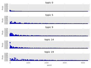

Finally, let's look at the topic distribution for a few documents. These distributions give the probability of each of the 20 topics for every document. I will only plot a few:

f, ax= plt.subplots(5, 1, figsize=(8, 6), sharex=True)
for i, k in enumerate([1, 3, 4, 8, 9]):
    ax[i].stem(doc_topic[k,:], linefmt='r-',
               markerfmt='ro', basefmt='w-')
    ax[i].set_xlim(-1, 21)
    ax[i].set_ylim(0, 1)
    ax[i].set_ylabel("Prob")
    ax[i].set_title("Document {}".format(k))

ax[4].set_xlabel("Topic")

plt.tight_layout()
plt.show()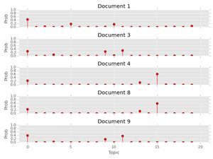

Plotting the distribution of topics for the above documents provides an important insight: many documents have more than one topic with high probability. As a result, choosing the topic with highest probability for each document can be subject to uncertainty; note to self: be careful. Maybe the full distribution over topics should be considered when comparing two documents?

That's it! As always, leave comments and questions below.