In this post I will expand on a previous example of inferring probabilities from a data series: Inferring probabilities, a second example of Bayesian calculations . In particular, instead of considering a discrete set of candidate probabilities, I'll consider all (continuous) values between \( 0 \) and \( 1 \). This means our prior (and posterior) will now be a probability density function (pdf) instead of a probability mass function (pmf). More specifically, I'll use the Beta Distribution for this example.

In the post Inferring probabilities, a second example of Bayesian calculations I considered inference of \( p_{0} \), the probability for a zero, from a data series:

\[ D = 0000110001 \]

I'll tackle the same question in this post using a different prior for \( p_{0} \), one that allows for continuous values between \( 0 \) and \( 1 \) instead of a discrete set of candidates. This makes the math a bit more difficult, requiring integrals instead of sums, but the basic ideas are the same.

This is one in a series of posts on Bayesian methods, starting from the basics and increasing in difficulty:

• Joint, conditional and marginal probabilities
• Medical tests, a first example of Bayesian calculations
• Inferring probabilities, a second example of Bayesian calculations

If the following is unfamiliar or difficult try consulting one or more of the above posts for some more basic, introductory material.

Likelihood

The starting point for our inference problem is the likelihood -- the probability of the observed data series, written like I know the value of \( p_{0} \) (see this post for more details, I'll be brief here):

\[ P(D=0000110001 \vert p_{0} ) = p_{0}^{7} \times (1-p_{0})^{3} \]

To be clear, we could plug in \( p_{0}=0.6 \), and find the probability of the specified data series given that value for the unknown probability:

\[ P(D=0000110001 \vert p_{0}=0.6 ) = 0.6^{7} \times (1-0.6)^{3} \]

A more general form for the likelihood, not being specific about the data series considered, is

\[ P(D \vert p_{0} ) = p_{0}^{n{0}} \times (1-p_{0})^{n_{1}} \]

where \( n_{0} \) is the number of zeros and \( n_{1} \) is the number of ones in whatever data series \( D \) is considered.

Prior -- The Beta Distribution

The new material, relative to the previous post on this topic, starts here. We use the Beta Distribution to represent our prior assumptions/information. The mathematical form is:

\[ P(p_{0} \vert \alpha_{0}, \alpha_{1} ) = \frac{ \Gamma(\alpha_{0} + \alpha_{1}) }{ \Gamma(\alpha_{0}) \Gamma(\alpha_{1}) } \, p_{0}^{\alpha_{0}-1} \, (1-p_{0})^{\alpha_{1}-1} \]

where \( \alpha_{0} \) and \( \alpha_{1} \) are hyper-parameters that we have to set to reflect our prior assumptions/information about the value of \( p_{0} \). I have found that a probability density funtion for a probability really confuses people. However, just think of \( p_{0} \) as a parameter that we want to infer-- ignore the fact that the parameter is a probability.

In any case, it is worth spending some time getting used to this prior and what it means. To help, I'll go though some properties of the Beta Distribution. However, note that the posterior pdf will also be a Beta Distribution, so it is worth the effort to get comfortable with the pdf.

So, some properties are (some of this material will be technical in nature, so skim it over at first and look at the Python code below if you find it too mathy):

Prior mean

Most people want a single number, or point estimate, to represent the results of inference or the information contained in the prior. However, in a Bayesian approach to inference the prior and posterior are both pdf's or pmf's. One way to get a point estimate is to take the average of the parameter of interest with respect to the prior or posterior. For example, for the Beta prior we obtain:

\[ \begin{eqnarray*} \mathbf{E}_{prior}[p_{0}] & = & \int_{0}^{1} \, dp_{0} \, p_{0} \, P(p_{0} \vert \alpha_{0}, \alpha_{1}) \\[1em] & = & \cfrac{\alpha_{0}}{\alpha_{0}+\alpha_{1}} \end{eqnarray*} \]

However, note that this single number does not fully characterize the prior or posterior and should be used with care. Many other properties (higher moments, variance, etc) can be calculated-- see Beta Distribution for more options. Also checkout this nice post on Probable Points and Credible Intervals for ideas on how to summarize a posterior distribution (also relevant to priors).

The prior pdf is normalized

This means if we integrate \( p_{0} \) from \( 0 \) to \( 1 \) we get one:

\[ \int_{0}^{1} \, dp_{0} \, P(p_{0} \vert \alpha_{0}, \alpha{1}) = 1 \]

This is true because of the following relationship:

\[ \int_{0}^{1} \, dp_{0} \, p_{0}^{\alpha_{0}-1} \, (1-p_{0})^{\alpha_{1}-1} = \frac{\Gamma(\alpha_{0}) \Gamma(\alpha_{1}) }{\Gamma(\alpha_{0} + \alpha_{1})} \]

The above integral produces the Beta function (the relation is also called the Euler integral). For our purposes, the most import information is the Beta Distribution is normalized on the \( 0 \) to \( 1 \) interval, as necessary for a probability like \( p_{0} \).

Prior assumptions and information

Prior assumptions and information can be reflected by setting hyper-parameters-- The hyper-parameters \( \alpha_{0} \) and \( \alpha_{1} \) affect the shape of the pdf, enabling a flexible encoding of prior information.

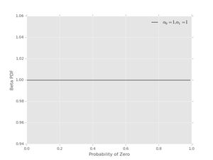
For example, no preferred values of \( p_{0} \) can be reflected by using \( \alpha_{0}=1 \), \( \alpha_{1}=1 \). This pdf looks like

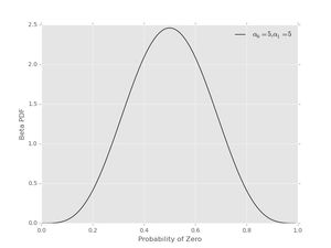
Another prior could assign \( \alpha_{0}=5 \), \( \alpha_{1}=5 \), which prefers values near \( p_{0}=1/2 \) and looks like

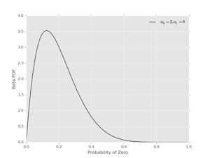
Finally, we can get non-symmetric priors using \( \alpha_{0} \neq \alpha_{1} \), as can be seen with \( \alpha_{0} = 2 \) and \( \alpha_{1} = 8 \)

Some things to remember about setting the hyper-parameters:

• If \( \alpha_{0}=\alpha_{1} \) the prior will be symmetric with prior mean equal to \( \mathbf{E}_{prior}[p_{0}] = 1/2 \).
• If \( \alpha_{0} \neq \alpha_{1} \) the prior will be asymmetric with a prior mean different from \( 1/2 \).
• The strength of the prior is related to the sum \( \alpha_{0} + \alpha_{1} \). Compare the alpha sum with \( n_{0} + n_{1} \) from the data, treating the alpha's as fake counts. The relative size of these sums controls the effects of the prior and likelihood on the shape of the posterior. This will become clear in the Python examples below.

The cumulative distribution function (cdf)

The cdf (see cumulative distribution function at wikipedia for more info) for the Beta Distribution gives the probability that \( p_{0} \) is less than or equal to a value \( x \). To be specific, the cdf is defined:

\[ \begin{array}{ll} P(p_{0} \leq x \vert \alpha_{0}, \alpha_{1}) & = & \int_{0}^{x} P(p_{0} \vert \alpha_{0}, \alpha_{1} ) \\[1em] & = & I_{x}(\alpha_{0}, \alpha_{1}) \end{array} \]

The integral is also called the incomplete Beta ingtegral and denoted \( I_{x}(\alpha_{0}, \alpha_{1}) \).

If we want the probability that \( p_{0} \) is between the values \( x_{l} \) and \( x_{h} \) we can use the cdf to calculate this:

\[ \begin{array}{ll} P(x_{l} \lt p_{0} \leq x_{h} \vert \alpha_{0}, \alpha_{1}) & = & P(p_{0} \leq x_{h} \vert \alpha_{0}, \alpha_{1}) \\[1em] & - & P(p_{0} \leq x_{l} \vert \alpha_{0}, \alpha_{1}) \\[1em] & = & I_{x_{h}}(\alpha_{0}, \alpha_{1}) - I_{x_{l}}(\alpha_{0}, \alpha_{1}) \end{array} \]

The incomplete Beta integral, or cdf, and it's inverse allows for the calculation of a credible interval from the prior or posterior. Using these tools the value of \( p_{0} \) can be said to be within a certain range with 95% probability-- again, we'll use Python code to plot this below.

The Beta Distribution is a conjugate prior for this problem-- This means that the posterior will have the same mathematical form as the prior (it will also be a Beta Distribution ) with updated hyper-parameters. This mathematical resonance is really nice and let's us do full Bayesian inference without MCMC.

Okay, enough about the prior and the Beta Distribution , now let's talk about Bayes' Theorem and the posterior pdf for this problem.

Bayes' Theorem and the Posterior

Our final goal is the posterior probability density function, combining the likelihood and the prior to make an updated reflection of our knowledge of \( p_{0} \) after considering data. The posterior pdf has the form (in this case):

\[ P(p_{0} \vert D, \alpha_{0}, \alpha_{1}) \]

In words, this is the probability density for \( p_{0} \) given data series \( D \) and prior assumptions, reflected by the Beta pdf with hyper-parameters* \( (\alpha_{0}, \alpha_{1}) \).

In this setting Bayes' Theorem takes the form:

\[ \color{blue}{P(p_{0} \vert D, \alpha_{0}, \alpha_{1})} = \frac{\color{black}{P(D \vert p_{0})} \color{red}{P(p_{0} \vert \alpha_{0}, \alpha_{1})} }{ \color{black}{\int_{0}^{1} \, d\hat{p}_{0} \, P(D \vert \hat{p}_{0})} \color{red}{P(\hat{p}_{0} \vert \alpha_{0}, \alpha_{1})} } \]

where

• the posterior \( \color{blue}{P(p_{0} \vert D, \alpha_{0}, \alpha_{1})} \) is blue,
• the likelihood \( P(D \vert p_{0}) \) is black,
• and the prior \( \color{red}{P(p_{0} \vert \alpha_{0}, \alpha_{1})}\) is red.

Notice that the normalizing marginal likelihood or evidence (denominator in the above equation) is now an integral. This is the price of using continuous values for \( p_{0} \)-- you should compare this with Bayes' Theorem in the Inferring probabilities, a second example of Bayesian calculations post.

As always, try to think about Bayes' Theorem as information about \( p_{0} \) being updated from assumptions ( \( \alpha_{0}, \alpha_{1} \) ) to assumptions + data ( \(D, \alpha_{0}, \alpha_{1} \) ):

\[ \color{red}{P(p_{0} \vert \alpha_{0}, \alpha_{1})} \rightarrow \color{blue}{P(p_{0} \vert D, \alpha_{0}, \alpha_{1})} \]

To get the posterior pdf, we have to do the integral in the denominator of Bayes' Theorem. In this case, the calculation is possible, using the properties of the Beta Distribution . The integral goes as follows:

\[ \begin{array}{ll} P(D \vert \alpha_{0}, \alpha_{1}) & = & \int_{0}^{1} \, d\hat{p}_{0} \, P(D \vert \hat{p}_{0}) P(\hat{p}_{0} \vert \alpha_{0}, \alpha_{1}) \\[1em] & = & \int_{0}^{1} \, d\hat{p}_{0} \, \hat{p}_{0}^{n_{0}} \, (1-\hat{p}_{0})^{n_{1}} \\[1em] & \times & \cfrac{ \Gamma(\alpha_{0} + \alpha_{1}) }{ \Gamma(\alpha_{0}) \Gamma(\alpha_{1}) } \hat{p}_{0}^{\alpha_{0}-1} (1-\hat{p}_{0})^{\alpha_{1}-1} \\[1em] & = & \cfrac{ \Gamma(\alpha_{0} + \alpha_{1}) }{ \Gamma(\alpha_{0}) \Gamma(\alpha_{1}) } \\[1em] & \times & \int_{0}^{1} \, d\hat{p}_{0} \, \hat{p}_{0}^{\alpha_{0}+n_{0}-1} \, (1-\hat{p}_{0})^{\alpha_{1}+n_{1}-1} \end{array} \]

The integral on the last line defines a Beta function , as discussed in the section on the prior, and has a known result:

\[ \int_{0}^{1} \, dp_{0} \, p_{0}^{\alpha_{0}+n_{0}-1} \, (1-p_{0})^{\alpha_{1}+n_{1}-1} = \frac{\Gamma(\alpha_{0}+n_{0}) \Gamma(\alpha_{1}+n_{1}) }{\Gamma(\alpha_{0} + \alpha_{1} + n_{0} + n_{1})} \]

This means the denominator, also called the marginal likelihood or evidence, is equal to:

\[ \begin{array}{ll} P(D \vert \alpha_{0}, \alpha_{1}) & = & \cfrac{ \Gamma(\alpha_{0} + \alpha_{1}) }{ \Gamma(\alpha_{0}) \Gamma(\alpha_{1}) } \\[1em] & \times & \cfrac{\Gamma(\alpha_{0}+n_{0}) \Gamma(\alpha_{1}+n_{1}) }{ \Gamma(\alpha_{0} + \alpha_{1} + n_{0} + n_{1})} \end{array} \]

If we plug all of this back into Bayes' Theorem we get another Beta Distribution for the posterior pdf, as promised above:

\[ \begin{array}{ll} P(p_{0} \vert D, \alpha_{0}, \alpha_{1} ) & = & \cfrac{ \Gamma(\alpha_{0} + \alpha_{1} + n_{0} + n_{1}) }{ \Gamma(\alpha_{0}+n_{0}) \Gamma(\alpha_{1}+n_{1}) } \\[1em] & \times & p_{0}^{\alpha_{0}+n_{0}-1} \, (1-p_{0})^{\alpha_{1}+n_{1}-1} \end{array} \]

Again, we obtain this result because the Beta Distribution is a conjugate prior for the Bernoulli Process likelihood that we are considering. Notice that the hyper-parameters from the prior have been updated by count data

\[ (\alpha_{0}, \alpha_{1}) \rightarrow (\alpha_{0}+n_{0}, \alpha_{1}+n_{1}) \]

This is exactly as one might expect without doing all of the math. In any case, before moving to implementing this in Python, a couple of notes:

• The posterior pdf is normalized on the \( 0 \) to \( 1 \) interval, just as we need for inferring a probability like \( p_{0} \).
• The posterior mean, a way to give a point estimate of our inference is

\[ \begin{array}{ll} \mathbf{E}_{post}[p_{0}] & = & \int_{0}^{1} \, dp_{0} \, p_{0} \, P(p_{0} \vert D, \alpha_{0}, \alpha_{1}) \\[1em] & = & \cfrac{\alpha_{0}+n_{0}}{\alpha_{0}+\alpha_{1}+n_{0}+n_{1}} \end{array} \]

• The cdf for the posterior is just like for the prior because we still have a Beta Distribution -- except, now the parameters are updated with data. In any case, we can find credible intervals with the incomplete Beta integral and it's inverse, as discussed above.

Inference code in Python

Note: code available as ex003_bayes.py at this gist (updated to gist Mar 5, 2015).

Let's do some Python. First, we do some import of packages that we will use to calculate and plot prior, likelihood and posterior. Notice that scipy.stats has a beta class that we will use for the prior and posterior pdfs. Also, we use matplotlib and the new styles, ggplot in this case, to create some nice plots with minimal tweaking.

from __future__ import division, print_function
import numpy as np
import matplotlib.pyplot as plt
from scipy.stats import beta

# use matplotlib style sheet
try:
    plt.style.use('ggplot')
except:
    # version of matplotlib might not be recent
    pass

Likelihood

The likelihood is exactly the same as for the previous example-- see Inferring probabilities, a second example of Bayesian calculations .

class likelihood:
    def __init__(self, data):
        """Likelihood for binary data."""
        self.counts = {s:0 for s in ['0', '1']}
        self._process_data(data)

    def _process_data(self, data):
        """Process data."""
        temp = [str(x) for x in data]
        for s in ['0', '1']:
            self.counts[s] = temp.count(s)

        if len(temp) != sum(self.counts.values()):
            raise Exception("Passed data is not all 0`s and 1`s!")

    def _process_probabilities(self, p0):
        """Process probabilities."""
        n0 = self.counts['0']
        n1 = self.counts['1']

        if p0 != 0 and p0 != 1:
            # typical case
            logpr_data = n0*np.log(p0) + \
                         n1*np.log(1.-p0)
            pr_data = np.exp(logpr_data)
        elif p0 == 0 and n0 != 0:
            # p0 can't be 0 if n0 is not 0
            logpr_data = -np.inf
            pr_data = np.exp(logpr_data)
        elif p0 == 0 and n0 == 0:
            # data consistent with p0=0
            logpr_data = n1*np.log(1.-p0)
            pr_data = np.exp(logpr_data)
        elif p0 == 1 and n1 != 0:
            # p0 can't be 1 if n1 is not 0
            logpr_data = -np.inf
            pr_data = np.exp(logpr_data)
        elif p0 == 1 and n1 == 0:
            # data consistent with p0=1
            logpr_data = n0*np.log(p0)
            pr_data = np.exp(logpr_data)

        return pr_data, logpr_data

    def prob(self, p0):
        """Get probability of data."""
        pr_data, _ = self._process_probabilities(p0)

        return pr_data

    def log_prob(self, p0):
        """Get log of probability of data."""
        _, logpr_data = self._process_probabilities(p0)

        return logpr_data

Prior

Our prior class will basically be a wrapper around scipy.stats.beta with a plotting method. Notice that the plot() method gets the Beta Distribution mean and uses the interval() method from scipy.stats.beta to get a region with 95% probability-- this is done, behind the scenes, using the incomplete Beta integral and it's inverse as discussed above.

class prior:
    def __init__(self, alpha0=1, alpha1=1):
        """Beta prior for binary data."""

        self.a0 = alpha0
        self.a1 = alpha1
        self.p0rv = beta(self.a0, self.a1)

    def interval(self, prob):
        """End points for region of pdf containing `prob` of the
        pdf-- this uses the cdf and inverse.

        Ex: interval(0.95)
        """

        return self.p0rv.interval(prob)

    def mean(self):
        """Returns prior mean."""

        return self.p0rv.mean()

    def pdf(self, p0):
        """Probability density at p0."""

        return self.p0rv.pdf(p0)

    def plot(self):
        """A plot showing mean and 95% credible interval."""

        fig, ax = plt.subplots(1, 1)
        x = np.arange(0., 1., 0.01)

        # get prior mean p0
        mean = self.mean()

        # get low/high pts containg 95% probability
        low_p0, high_p0 = self.interval(0.95)
        x_prob = np.arange(low_p0, high_p0, 0.01)

        # plot pdf
        ax.plot(x, self.pdf(x), 'r-')

        # fill 95% region
        ax.fill_between(x_prob, 0, self.pdf(x_prob),
                        color='red', alpha='0.2' )

        # mean
        ax.stem([mean], [self.pdf(mean)], linefmt='r-',
                markerfmt='ro', basefmt='w-')

        ax.set_xlabel('Probability of Zero')
        ax.set_ylabel('Prior PDF')
        ax.set_ylim(0., 1.1*np.max(self.pdf(x)))

        plt.show()

Let's plot some Beta pdfs with a range of parameters using the new code. First, the uniform prior

pri = prior(1, 1)
pri.plot()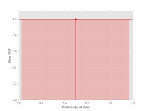

The vertical line with the dot shows the location of the mean of the pdf. The shaded region indicates the (symmetric) region with 95% probability for the given values of \( \alpha_{0} \) and \( \alpha_{1} \). If you want the actual values for the mean and the credible interval, these can be obtained as well:

print("Prior mean: {}".format(pri.mean()))
cred_int = pri.interval(0.95)
print("95% CI: {} -- {}".format(cred_int[0], cred_int[1]))

Prior mean: 0.5
95% CI: 0.025 -- 0.975

The other prior examples from above also work:

pri = prior(5, 5)
pri.plot()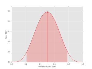

and

pri = prior(2, 8)
pri.plot()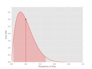

It's useful to get a feel for the mean and uncertainty of prior assumptions, as reflected by the hyper-parameters-- try out some other values to build an intuition.

Posterior

Finally, we build the class for the posterior. As you might expect, I'll take data and a prior as arguments and extract the parameters needed for the posterior from these elements.

class posterior:
    def __init__(self, data, prior):
        """The posterior.

        data: a data sample as list
        prior: an instance of the beta prior class
        """
        self.likelihood = likelihood(data)
        self.prior = prior

        self._process_posterior()

    def _process_posterior(self):
        """Process the posterior using passed data and prior."""

        # extract n0, n1, a0, a1 from likelihood and prior
        self.n0 = self.likelihood.counts['0']
        self.n1 = self.likelihood.counts['1']
        self.a0 = self.prior.a0
        self.a1 = self.prior.a1

        self.p0rv = beta(self.a0 + self.n0,
                         self.a1 + self.n1)

    def interval(self, prob):
        """End points for region of pdf containing `prob` of the
        pdf.

        Ex: interval(0.95)
        """

        return self.p0rv.interval(prob)

    def mean(self):
        """Returns posterior mean."""

        return self.p0rv.mean()

    def pdf(self, p0):
        """Probability density at p0."""

        return self.p0rv.pdf(p0)

    def plot(self):
        """A plot showing prior, likelihood and posterior."""

        f, ax= plt.subplots(3, 1, figsize=(8, 6), sharex=True)
        x = np.arange(0., 1., 0.01)

        ## Prior
        # get prior mean p0
        pri_mean = self.prior.mean()

        # get low/high pts containg 95% probability
        pri_low_p0, pri_high_p0 = self.prior.interval(0.95)
        pri_x_prob = np.arange(pri_low_p0, pri_high_p0, 0.01)

        # plot pdf
        ax[0].plot(x, self.prior.pdf(x), 'r-')

        # fill 95% region
        ax[0].fill_between(pri_x_prob, 0, self.prior.pdf(pri_x_prob),
                           color='red', alpha='0.2' )

        # mean
        ax[0].stem([pri_mean], [self.prior.pdf(pri_mean)],
                   linefmt='r-', markerfmt='ro',
                   basefmt='w-')

        ax[0].set_ylabel('Prior PDF')
        ax[0].set_ylim(0., 1.1*np.max(self.prior.pdf(x)))

        ## Likelihood
        # plot likelihood
        lik = [self.likelihood.prob(xi) for xi in x]
        ax[1].plot(x, lik, 'k-')
        ax[1].set_ylabel('Likelihood')

        ## Posterior
        # get posterior mean p0
        post_mean = self.mean()

        # get low/high pts containg 95% probability
        post_low_p0, post_high_p0 = self.interval(0.95)
        post_x_prob = np.arange(post_low_p0, post_high_p0, 0.01)

        # plot pdf
        ax[2].plot(x, self.pdf(x), 'b-')

        # fill 95% region
        ax[2].fill_between(post_x_prob, 0, self.pdf(post_x_prob),
                           color='blue', alpha='0.2' )

        # mean
        ax[2].stem([post_mean], [self.pdf(post_mean)],
                   linefmt='b-', markerfmt='bo',
                   basefmt='w-')

        ax[2].set_xlabel('Probability of Zero')
        ax[2].set_ylabel('Posterior PDF')
        ax[2].set_ylim(0., 1.1*np.max(self.pdf(x)))

        plt.show()

That's it with the base code, let do some examples.

Examples

Let's start with an example using the data at the start of the post and a uniform prior. You can also compare the result with example from the previous post using a set of candidate probabilities-- Inferring probabilities, a second example of Bayesian calculations .

# data
data1 = [0,0,0,0,1,1,0,0,0,1]

# prior
prior1 = prior(1, 1)

# posterior
post1 = posterior(data1, prior1)
post1.plot()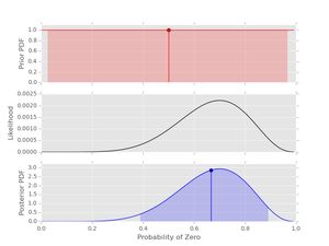

Things to note here:

• The prior is uniform. This means that the likelihood and the posterior have the same shape.
• The 95% credible interval is shown for both the prior and the posterior-- note how the information about \( p_{0} \) has been updated with this short data series.

Next, let's consider the same data with a prior that is not uniform. The dataset is length 10, so \( n_{0}+n_{1}=10 \). Let's set a prior with \( \alpha_{0}+\alpha_{1}=10 \) but the prior is peaked in a different location from the likelihood (maybe an expert has said this should be the prior setting):

# prior
prior2 = prior(4, 6)

# posterior
post2 = posterior(data1, prior2)
post2.plot()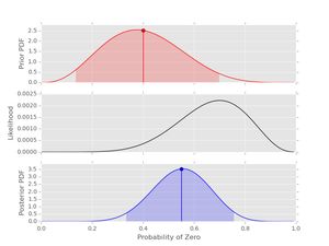

Well, obviously the data and the expert disagree at this point. However, because the prior is set with weight 10 and the data series is length 10 the posterior peaks midway between the peaks in the prior and likelihood. Try playing with this effect to better understand the interplay between the prior hyper-parameters, the length of the dataset and the resulting posterior.

As a final example we consider two variants of the last example from Inferring probabilities, a second example of Bayesian calculations . First we use a uniform prior:

# set probability of 0
p0 = 0.23
# set rng seed to 42
np.random.seed(42)
# generate data
data2 = np.random.choice([0,1], 500, p=[p0, 1.-p0])

# prior
prior3 = prior(1,1)

# posterior
post3 = posterior(data2, prior3)
post3.plot()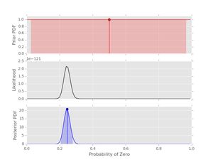

Notice that the likelihood and posterior peak in the same place, just as we would expect. However, the peak is much stronger due to the longer dataset (500 values).

Finally we use a 'bad prior' on the same dataset. In this case we'll keep the strength of the prior at 10, that is \( \alpha_{0}+\alpha_{1}=10 \):

# prior
prior4 = prior(6,4)

# posterior
post4 = posterior(data2, prior4)
post4.plot()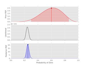

Notice that the likelihood and posterior are very similar despite the prior that peaks in the wrong place. This examples demonstrates that a reasonable amount of data should produce decent inference if the prior has not been set too strong. In general it's good to have \( n_{0}+n_{1} \gt \alpha_{0} + \alpha_{1} \) and to consider the shapes of both the prior and posterior.

That's it for this post. As always, comments, questions, and corrections as welcome!